Hardware drift ranges¶

Robustness numbers only mean something against a drift range the hardware actually shows. This page fixes those ranges from measurements on fixed-frequency transmons, the qubit type in our model. They are encoded in rlquantopt/jx/drift.py and used for robust GRAPE, for scoring pulses, and for domain randomisation.

The three ranges¶

Range	Half-width on each qubit	Timescale	Evidence
In-cooldown	±0.1 MHz	hours to days	Frequencies "remain generally stable with variations confined to a 100 kHz-interval" over 95 h (Dhieb et al. 2025). Single two-level-system (TLS) fluctuators shift the qubit by 5-140 kHz (Schlör et al., PRL 123, 190502 (2019)). Typical shifts of 1-3 kHz, infrequently up to 20 kHz, over several days (Burnett et al., npj QI 5, 54 (2019)).
Recool	±5.7 MHz	between cooldowns	"Cryogenic-to-ambient thermal cycling … yields a recool stability of 5.7 MHz" on IBM multi-qubit processors (Zhang et al., Sci. Adv. 8, eabi6690 (2022)).
Fabrication targeting	±18.5 MHz	a new device	"Frequency assignment precision of 18.5 MHz" after laser annealing, including pre-cooldown steps (Zhang et al. 2022).

The sources report spreads (a precision or a stability), not hard bounds. We use each number as the half-width of a uniform box on both qubits, which covers roughly ±1σ; the worst case over the box is therefore a typical bad case, not an extreme one.

What they imply for this project¶

In-cooldown drift is negligible for our gates. 0.1 MHz over a 17 ns gate is a phase error of \(2\pi \times 0.1\,\text{MHz} \times 17\,\text{ns} \approx 0.01\) rad. Every pulse we have keeps its nominal J_T across this range (see Robustness).
Recool drift is the relevant range for robustness. Pulses must survive a thermal cycle without re-optimisation. 5.7 MHz is 0.11 % of 5.0311 GHz and 0.10 % of 5.8899 GHz, so the paper's ±0.1 % domain randomisation corresponds to this range.
Fabrication targeting is the range for transfer between devices. A policy that works across ±18.5 MHz could be reused on a new chip without retraining. That is where a trained policy can beat per-device optimisation.
The paper's ±50 MHz maps (Figs. 10-17) cover about 2.7× the fabrication-targeting range. They show the shape of the landscape but overstate the drift a calibrated device sees.

Where the ranges are used¶

Range	Used for	Result
In-cooldown ±0.1 MHz	Scoring pulses	No re-calibration needed within a cooldown (Robustness)
Recool ±5.7 MHz	Robust-GRAPE ensemble; domain randomisation of the RL agent (`--max-drift 1.1e-3`); the 24 test devices of the cost-per-device experiment	Robust GRAPE survives a recool; single pulses do not (Robustness)
Fabrication ±18.5 MHz	Scoring transfer to a new device; the fabrication-range experiment	A robust pulse trained on this range covers it (Robustness)
Coupler ±140 MHz (worst-loop flux drift)	Large coupler drift experiment; gecko and ibis	Robustness, Measurable, ibis
Coupler flux ±20 mΦ₀ with qubits ±5.7 MHz (physical units)	The realistic device model	jackal

What is not covered yet¶

The coupler drifts too, and more¶

The coupler is flux-tunable, and flux-tunable elements are much less stable than fixed-frequency qubits: Burnett et al. (2019) contrast their kHz-level drift with "the approximately 500 kHz frequency instability found in flux-tuneable qubits". Over days and weeks the flux offset itself wanders. Dai et al. (2021) measured, on a device kept cold: "After two days, the root mean square (RMS) change in flux offsets […] is 1.3 mΦ0. After 17 days, one of the resonator SQUID fluxes changed by 20.0 mΦ0. The others have an RMS change of 2.0 mΦ0."

Turning flux into coupler frequency needs the coupler's flux map, which the paper's model does not have. Assuming a symmetric-SQUID coupler with a maximum frequency of 8 GHz, parked at our 7.445 GHz (about 6.8 MHz per mΦ0 there):

Flux drift [Dai et al. 2021]	Coupler frequency drift (assumed f_max = 8 GHz)
1.3 mΦ0 RMS, after 2 days	±9 MHz
2.0 mΦ0 RMS, after 17 days	±14 MHz
20 mΦ0, worst loop after 17 days	−144 / +127 MHz, used as ±140 MHz

A higher f_max, or parking further from the sweet spot, makes the slope and the drift larger.

In flux units: the realistic device model

The jackal device model (i10) has the coupler's flux map (an asymmetric SQUID, Sung et al. 2021 parameters), so its drift is drawn directly in flux, up to ±20 mΦ₀ (about −178 MHz of coupler frequency at its idle point), together with the qubit frequencies (±5.7 MHz) and, optionally, the couplings and anharmonicities, which a spectroscopy calibration does not measure.

In the paper's model the coupler term is \(2\pi(\omega_c - \omega_r) b^\dagger b + u(t)\, b^\dagger b\), so a coupler drift \(\delta\) is exactly a static offset \(2\pi\delta\) on the control line. How far each pulse tolerates it (scripts/coupler_drift_scan.py):

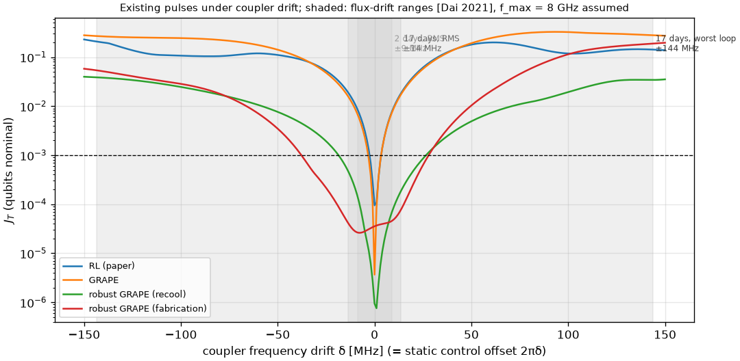
Pulse	Coupler window with J_T ≤ 1e-3
RL (paper)	5 MHz wide
GRAPE	6 MHz wide
Robust GRAPE, recool ensemble (qubits only)	44 MHz wide
Robust GRAPE, fabrication ensemble (qubits only)	64 MHz wide

Typical weeks-scale coupler drift (±14 MHz) is covered by the robust pulses although they never saw coupler drift. The worst-loop drift (±140 MHz) breaks every existing pulse, and is used for the large coupler drift experiment.

Further sources of slow drift, not modelled: aging of junctions across many cooldowns (a cumulative ~61 MHz downward shift over more than a year and 10 thermal cycles in Dhieb et al. 2025), and calibration drift of the control electronics.

Using the ranges in code¶

from rlquantopt.jx.drift import DRIFT_RANGES, box_grid
rng = DRIFT_RANGES["recool"]                  # DriftRange(name, half_width_mhz=5.7, timescale, source)
d0, d1 = box_grid(rng.half_width_mhz, 11)     # MHz grid for scoring a pulse
omegas = grape.detuning_grid(model, rng.half_width_mhz, 5)   # ensemble for robust GRAPE

For training with domain randomisation, --max-drift is a fraction of each frequency: --max-drift 1.1e-3 gives ±5.5 MHz on qubit 0 and ±6.5 MHz on qubit 1, approximately the recool range.