🦩 i09 ibis: gecko made data-lean

🏁 concluded 2026-09-26, v2.19.0 · positive: an open-loop policy fed only a frequency calibration gives 1 − F ≈ 4e-3 on every drifted device, 4 seeds, robust to 10× calibration errors · continued by jackal

Runs in runs/i09_ibis/, records in results/i09_ibis/. Continued on a realistic device model in jackal.

Answer so far. Yes, with the right action space. A policy that steers a carrier at the qubit detuning (amplitude, phase, offset) and sees only a routine frequency calibration, measured once before the pulse, plays the whole pulse open loop and reaches 1 − F = 3.9e-3 (median; all 24 drifted devices below 1e-2) with about 1e4 shots per device. It learns 11× faster than the best closed-loop policy and beats it, even when that one gets exact observations. See the carrier.

Question. Can everything be done, if necessary, on a real machine with its own observables, using as little data as possible? Concretely: how few measurement shots per pulse and how small a policy network still give a good gate under the large coupler drift (qubits ±5.7 MHz, coupler ±140 MHz), with the √iSWAP fidelity of gecko?

Design

Ingredient	What it does	Flag
Clip instead of terminate	An amplitude beyond ±20 rad/ns is clipped and costs oob_penalty per unit of excess; the episode goes on, so the policy never loses its pulse (gecko's two failed devices)	--oob-mode clip --oob-penalty λ
Finite shots	Each observed value is estimated from N shots per measurement setting (multinomial over the readout outcomes); one step costs 30 settings, i.e. 30 N shots	--shots N
Smaller networks, GELU	Hidden widths and activation	--hidden 64 64 --activation gelu
Longer steps	K samples per step (fewer, longer steps: fewer experiments per episode); the per-sample action scale must shrink with K	--n-time-steps 15 --delta-scale 4
Calibration context	The policy sees the qubit and coupler frequency offsets, measured once before the pulse (spectroscopy, error 0.1 / 0.1 / 1 MHz), with or without the measured observables	--obs-mode context / measured+context
Fidelity from measured data	The √iSWAP fidelity (free Z) reconstructed from the 30 settings alone: magnitudes from populations, phases from Pauli expectations; no Hamiltonian	metrics.fidelity_from_observables
Model-free refinement	SPSA and CMA-ES on that estimate, every shot counted	rlquantopt/jx/refine.py
Carrier action	u(t) = offset + A cos(2π f_d t + φ); the policy nudges (A, φ, offset); f_d = nominal qubit detuning, corrected by the measured calibration	--action-mode carrier

The quality of a policy is now the full pulse (the last step). Cutting the pulse at its best step, as in gecko, needs the exact fidelity, which a lab does not have.

Results so far

Policies trained on exact observations, deployed with finite shots

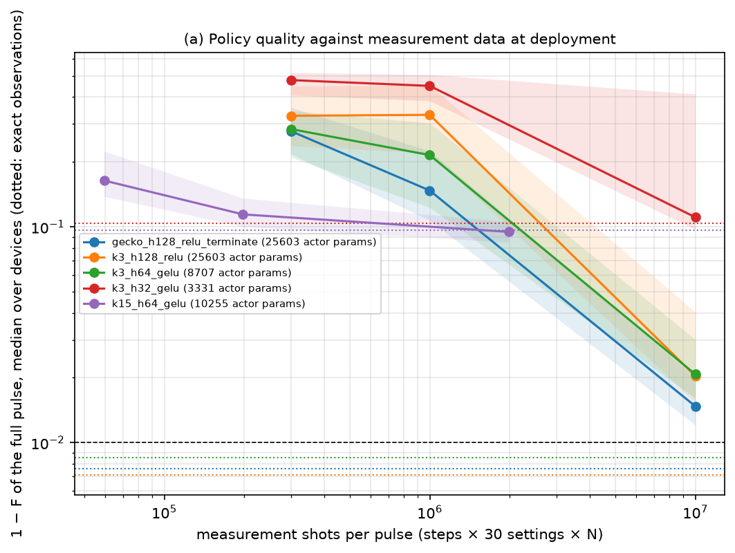
scripts/ibis_eval.py: the same 24 held-out devices as gecko, 1 − F of the full pulse, median over devices (3 noise draws per device), for N shots per setting at deployment.

Policy	Actor params	Exact	N = 1000 (1e7 shots/pulse)	N = 100 (1e6)	N = 30 (3e5)	Env steps to 1e-2
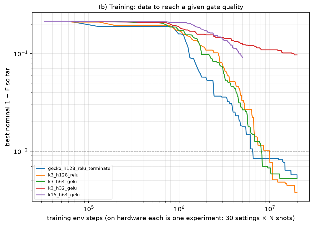
gecko: 128×128 ReLU, terminate	26k	7.6e-3	1.5e-2	1.5e-1	2.8e-1	6.6M
128×128 ReLU, clip λ = 1	26k	7.1e-3	2.0e-2	3.3e-1	3.3e-1	9.9M
64×64 GELU, clip λ = 1	8.7k	8.5e-3	2.1e-2	2.2e-1	2.8e-1	8.1M
32×32 GELU, clip λ = 1	3.3k	1.0e-1	1.1e-1	4.5e-1	4.8e-1	never
K = 15, 64×64 GELU (5M steps)	8.7k	9.7e-2	9.5e-2	1.1e-1	1.6e-1	never

1. Closed-loop policies trained on exact data do not survive shot noise. At 1e6 shots per pulse they are 30× worse: they react to each of 333 noisy observations and the errors compound.
2. 64×64 GELU matches 128×128 ReLU with a third of the actor parameters and reaches 1e-2 in fewer steps than the clip-mode ReLU network; 32×32 is too small for this task.
3. λ = 1 is too weak: 5-9 % of the steps are still clipped with exact observations.
4. Longer steps (K = 15) are robust to noise but poor (about 0.1). With v1's per-sample action scale they did not learn at all (every exploration hit the bound, the agent settled on the identity); --delta-scale 4 fixed that, but 5M steps were not enough.

Refinement from measured data only

The fidelity estimate from the 30 measured settings equals the true fidelity on exact data (to the digits printed, on GRAPE and random pulses: the neglected coupler coherences do not matter); with N = 1000 it resolves infidelities down to about 5e-4 (spread ±4e-4, a small upward bias).

But black-box refinement of a policy pulse barely moves it. Noise-free, 1500 fidelity estimates:

Correction basis	Start	CMA-ES	SPSA
3 physical knobs (offset, AC scale, ramp) + 8 sine modes	5.8e-3	4.0e-3	5.3e-3
24 sine modes (≤ 0.24 GHz)	5.8e-3	4.3e-3	5.0e-3
100 sine modes (≤ 1 GHz)	5.8e-3	3.7e-3	4.5e-3

(one device; a second one gives the same picture). With N = 1000 shots it is worse. GRAPE reaches 1e-8 from the same pulses because it gets the exact gradient in all 999 samples at every step; a black-box optimiser has to discover that information one noisy fidelity at a time. The gradient is not the issue: 57-81 % of its power sits below 0.25 GHz, inside the bases above. So the policy must be good enough on its own, which is what the current runs address.

The carrier: steer slow knobs, not samples

The calibration-only policy above could not learn with per-sample actions: it sat at the identity gate (0.22) for 20M steps, whatever the penalty. A good pulse rides on a carrier near the qubit-qubit detuning, about 0.86 GHz (43 periods in 50 ns); a closed-loop policy can pick up that rhythm from the rotating state it observes, but an open-loop policy sees only a clock and cannot synthesise 43 oscillations from it. Giving it the carrier, as a lab drives a gate, fixes this: the action nudges the amplitude, phase and offset of u(t) = offset + A cos(2π f_d t + φ). Four constant knobs alone already reach 1.9e-3 at 50 ns, so shaping them over time has room below 1e-3.

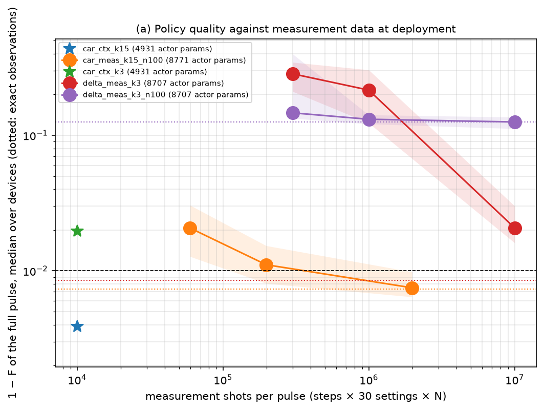
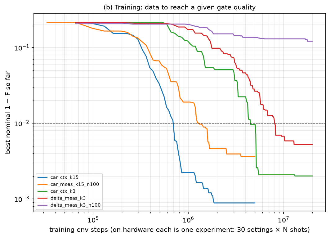
All 64×64 GELU, clip λ = 1; 24 drifted devices, full pulse:

Policy	Shots per device	1 − F median [quartiles]	Below 1e-2	Env steps to 1e-2 (nominal)
Carrier, calibration only, K = 15 (open loop)	1e4 (calibration)	3.9e-3 [2.5e-3, 4.4e-3]	100 %	0.72M
Carrier, calibration only, K = 3	1e4	2.0e-2 [7.5e-3, 1.0e-1]	38 %	4.5M
Carrier, measured, trained with N = 100, K = 15	2e6 (N = 1000) / 2e5 (N = 100) / 6e4 (N = 30)	7.5e-3 / 1.1e-2 / 2.1e-2	81 % / 42 % / 11 %	1.3M
Carrier, measured, K = 3 (exact or N = 100)		stuck at 0.21	0 %	never
Per-sample, measured, exact-trained, K = 3 (the best before)	1e7 (N = 1000)	8.5e-3 exact, 2.1e-2 at N = 1000	75 % exact, 3 % at N = 1000	8.1M
Per-sample, measured, trained with N = 100, K = 3	1e6 (N = 100)	1.3e-1	0 %	never

1. The open-loop carrier policy is the best on every axis: lower infidelity than the best closed-loop policy with exact observations, about 1000× fewer shots than a closed-loop policy at N = 1000, and 11× fewer training steps. The calibration it needs (qubit and coupler frequencies, with 0.1 / 0.1 / 1 MHz errors) is what a lab measures routinely; it does not need the Hamiltonian.
2. With the carrier, closed loop with shot noise works too: 1.1e-2 at 2e5 shots per pulse, 20× better than the per-sample policy trained with the same noise.
3. Few, long steps matter in carrier mode: K = 3 (333 small knob decisions) learns badly or not at all; K = 15 (66 decisions) learns within 1M steps.

Closing tests: seeds, calibration stress, unseen drift, size, step length

All carrier, calibration only, 64×64 GELU (unless noted), clip λ = 1, 5M steps; the same 24 drifted devices, full pulse. Script: scripts/ibis_eval.py (and --stress).

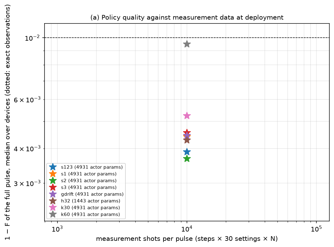
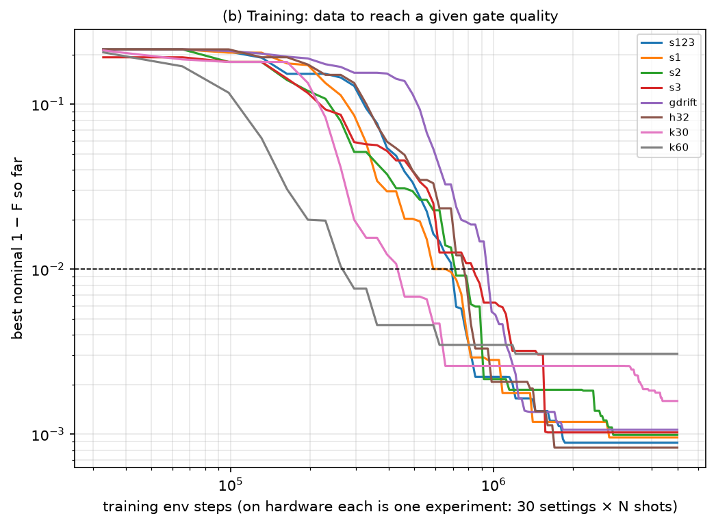
Policy	Actor params	1 − F, median	Below 1e-2	Env steps to 1e-2 (nominal)
K = 15, seed 123	4.9k	3.9e-3	100 %	0.72M
K = 15, seed 1	4.9k	4.4e-3	100 %	0.69M
K = 15, seed 2	4.9k	3.7e-3	100 %	0.72M
K = 15, seed 3	4.9k	4.6e-3	100 %	0.85M
K = 15, couplings also drift in training (±5.7 MHz)	4.9k	4.5e-3	100 %	0.95M
K = 15, 32×32	1.4k	4.3e-3	100 %	0.79M
K = 30 (33 decisions)	4.9k	5.2e-3	100 %	0.46M
K = 60 (16 decisions)	4.9k	9.5e-3	67 %	0.29M

Calibration stress (median 1 − F over the four K = 15 seeds, and the share of device × noise draws below 1e-2):

Calibration at deployment	Devices as in training	Couplings (±5.7 MHz) and anharmonicities (±5 MHz) also drift, unseen
Errors as in training (0.1 / 0.1 / 1 MHz)	3.7-4.7e-3, 100 %	3.8-4.8e-3, 99-100 %
3× larger	3.7-4.6e-3, 100 %	3.9-4.8e-3, 97-100 %
10× larger (1 / 1 / 10 MHz)	4.2-5.1e-3, 92-99 %	4.4-5.0e-3, 86-96 %
Stale (fixed bias +0.3 / −0.3 / +5 MHz) + 10× errors	4.4-5.8e-3, 81-99 %	4.3-6.0e-3, 78-93 %

1. The result is reproducible. Four seeds give 3.7-4.6e-3 on the drifted devices, all below 1e-2, and reach 1e-2 in 0.69-0.85M training steps.
2. It is robust to the calibration. Ten times larger frequency errors than in training raise the median infidelity by 0-15 %; a stale calibration on top costs a little more. Drift the calibration does not see (couplings, anharmonicities) barely matters here, and training with coupling drift makes the policy the most robust of all (94-100 % below 1e-2 in every case).
3. Small is enough. A 32×32 policy with 1.4k actor parameters matches the 64×64 one.
4. Fewer decisions are cheaper to learn but cost quality. 33 decisions (K = 30) reach 1e-2 fastest among the good policies (0.46M steps) at 5.2e-3; 16 decisions (K = 60) reach it in 0.29M steps but end at 9.5e-3.

Conclusion

In the paper's model, under large coupler drift, a pulse needs neither the Hamiltonian nor measurements during the pulse: an open-loop policy of 1.4-4.9k parameters, fed only a routine frequency calibration and steering the knobs of a carrier, gives 1 − F ≈ 4e-3 on every drifted device with about 1e4 shots of calibration, robust to calibration errors ten times larger than in training. It learns in under 1M simulated steps. The closed-loop, measurement-driven policies of the first half of ibis could not approach this with 1e7 shots per pulse. The MDP is described on The calibration policy (new MDP); whether it survives a realistic device is the question of jackal.

Next (in jackal)

1. The realistic device: no RWA, direct coupling, flux-tunable coupler, AWG and flux-line filter, physical drift (jackal).
2. Decoherence, a final-pulse reward for training on hardware, and a Bayesian tune-up after deployment.