Drift, dimension and learned policies

This page states the project's central hypothesis, sharpens it into claims that can be tested, collects what the literature and our own experiments say for and against each claim, and lists the experiments that would settle it. It is a working document: a claim moves to "supported" only when the evidence below supports it.

The hypothesis

Environment drift blows up the space a controller has to cover faster than, and in proportion to, the dimensional size of the problem. Finding a policy with reinforcement learning is therefore informationally far more efficient than gradient-derived techniques once theory meets the limits of real hardware.

The intuition: a gradient method returns one pulse for one device state. When the device drifts, it must be run again. A policy maps the device state to a pulse, so it answers every future calibration at once. If the number of calibrations a device needs grows quickly with the number of things that can drift, the policy's up-front cost is paid back more and more quickly.

To test it, we split it into three claims.

Claim	Statement	Status
H1: drift multiplies the problem	The number of distinct calibrations needed to keep a gate below an error target over a drift range grows multiplicatively with the number of sensitive drifting parameters, and that number grows with the size of the processor.	Partly supported: multiplicative over sensitive parameters, but in the two-qubit model one robust pulse still covers ±18.5 MHz
H2: policies amortise	A policy trained over the drift distribution produces a good pulse for a new device state at a small fraction of the cost of re-optimising, so its total cost wins beyond some number of calibrations.	Supported as a warm start, at matched gate time (1-3 orders of magnitude better than a random start at equal GRAPE budget); not supported for the policy alone, which does not reach J_T ≤ 1e-3
H3: hardware limits favour policies	On hardware, gradients must be estimated from measurements, at a cost that grows with the number of pulse parameters and the shot noise, which removes most of the advantage gradient methods have in simulation.	Supported by the literature in principle; not yet tested here

What the literature says

Drift is a real, recurring cost. Optimal control parameters "are typically different between devices and can also drift in time, which begets the need for an efficient calibration strategy" [kelly2018]. Errors "typically fluctuate over time", and tools that assume static errors cause "unheralded failures" and "wasted experimental effort" [proctor2020]. Our own drift ranges put numbers on this for transmons: kHz within a cooldown, 5.7 MHz across a thermal cycle, 18.5 MHz between devices [zhang2022].

Calibration scales badly with processor size (H1). Scaling gates to large processors "often maps to non-convex, high-constraint, and time-dependent control optimization over an exponentially expanding configuration space" [klimov2024]. This is the strongest published support for H1, for joint frequency configurations of a whole processor.

Amortisation can be orders of magnitude faster, after training (H2). Learning to predict solutions across related problem instances can "solve optimization problems many orders of magnitude faster than traditional optimization methods that don't use amortization" [amos2023]. This is the precise sense in which "orders of magnitude" is defensible: per new instance, once the model is trained, not in total and not for one instance.

Gradients on hardware are expensive (H3). Analytic gradients of a quantum circuit can be estimated on hardware, but each parameter needs its own shifted evaluations [schuld2019], so the cost of one gradient grows with the number of parameters (345 per pulse here), times the shots needed to resolve an error of 1e-4. Hybrid schemes that combine a model with measured data exist, precisely because model gradients alone miss the real device: Ad-HOC [egger2014] and data-driven GRAPE using tomography [wu2018].

What the literature contradicts. For a single problem instance, methods that only see function values (as model-free RL does with rewards) are provably slower than gradient methods. For convex problems, such methods "usually need at most n times more iterations than the standard gradient methods, where n is the dimension of the space of variables" ([nesterov2017], abstract). Gate optimisation is not convex, so the bound is a guide rather than a theorem here, but the direction is clear: here n = 345 pulse samples. So "RL is orders of magnitude more efficient than any gradient technique" is false per instance. Our own data agree: GRAPE needs 14 core-seconds per device, while training the RL agent took 0.81 core-hours, about 200 times more.

What can and cannot be claimed

The defensible claim is about total cost over many drifting device states, and about settings where exact gradients are not available (hardware). It is not a general claim that policy search beats gradient descent.

Evidence from our experiments

H1: coverage as more parameters drift

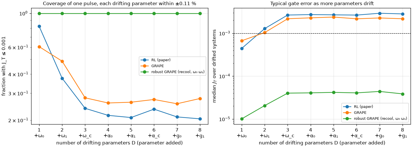
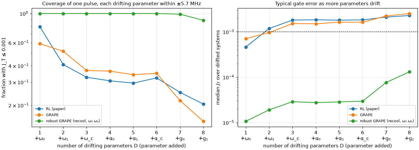
One pulse, optimised for the nominal device, is evaluated on 1,000 drifted systems as the number of drifting parameters D grows, adding them in the order ω₀, ω₁, ω_c, α₀, α₁, α_c, g₀, g₁. The left figure uses the recool spread for every parameter as a fraction of its value (±0.11 %; measured for the qubit frequencies, assumed for the rest). The right figure is a stylised stress test in which every parameter drifts by the same ±5.7 MHz.

Pulse	Covered (J_T ≤ 1e-3), D = 1 → 3 → 8, relative drift	Same, ±5.7 MHz on every parameter
RL (paper)	82 % → 24 % → 20 %	80 % → 33 % → 20 %
GRAPE (nominal)	61 % → 28 % → 28 %	59 % → 37 % → 15 %
Robust GRAPE (trained on ω₀, ω₁)	100 % → 100 % → 100 %	100 % → 100 % → 89 %

What this shows:

• Coverage falls multiplicatively, but only over sensitive directions. Each qubit or coupler frequency that drifts removes a large share of the coverage. At realistic relative drift, the anharmonicities and couplings move by only 0.1-0.4 MHz and barely matter, so coverage flattens after D = 3. The number that matters is the effective dimension: the drifting parameters the gate is sensitive to.
• Robustness does not transfer to directions it was not trained on. Robust GRAPE, whose ensemble covers only ω₀ and ω₁, loses coverage once the couplings drift by ±5.7 MHz (D = 7, 8). Every sensitive drifting parameter must be in the ensemble, and a grid ensemble with m points per parameter has m^D members, which makes robust optimisation exponentially costly in D.
• For H1 on a whole processor the effective dimension grows with the number of qubits and couplers, since each has its own frequency. For a strictly local two-qubit gate, only its own neighbourhood matters; the exponential growth [klimov2024] describes arises from the joint configuration of many gates and from crosstalk. A three-qubit model with a spectator is needed to test this here.

H2: amortisation

From Robustness: cost per device:

• A PPO agent trained over the recool drift gives consistent gates on every held-out device, and as a warm start it cuts GRAPE's per-device compute 15× (0.94 vs 14 core-seconds).
• Its training (0.81 core-hours) pays back after ≈ 220 devices or recalibrations (≈ 350 over the fabrication range, where the policy's longer pulses make each refinement step dearer).
• Within the recool range, and even over the ±18.5 MHz fabrication range, a single robust GRAPE pulse covers two drifting frequencies (fabrication-range experiment).
• At matched gate time, the policy's pulse is a far better GRAPE starting point than a random guess: 1-3 orders of magnitude lower J_T at equal GRAPE budget. A policy trained for only 2M steps is already a good warm start, which moves the break-even to about 36 devices.

T1: policies trained with more drifting parameters

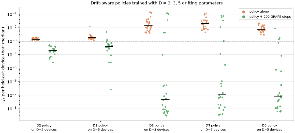
Three PPO policies (seed 123, 20M steps each) trained with drift redrawn every episode over D = 2 (both qubit frequencies, ±0.11 %), D = 3 (+ coupler frequency, ±5.7 MHz) and D = 5 (+ both couplings, ±5.7 MHz), tested on the same 24 held-out devices drifting in D = 5 (and in their own dimensions). Script: scripts/drift_dimension_policies.py.

Policy	Tested on	Policy alone: median J_T	+ 200 GRAPE steps: median J_T	Reach 1e-3	Median gate time
D = 2	D = 2 devices	1.4e-3	2.0e-4	100 %	38 ns
D = 2	D = 5 devices	1.8e-3	4.0e-4	92 %	36 ns
D = 3	D = 3 devices	1.4e-2	5.0e-8	79 %	40 ns
D = 3	D = 5 devices	2.0e-2	1.2e-7	75 %	41 ns
D = 5	D = 5 devices	7.0e-3	8.3e-8	88 %	42 ns

Control on the D = 5 devices: GRAPE from a random guess at each device's D = 5 gate time reaches a median of 1.1e-2 after 200 steps (0 % below 1e-3) and 8.1e-5 after 500 (92 %).

What T1 shows, honestly:

• At equal budget, training over more drifting parameters made the policy alone worse (1.4e-3 for D = 2 against 7.0e-3-1.4e-2 for D = 3 and 5, on their own devices). That fits the hypothesis that drift dimensions make the control problem harder.
• But the D = 2 policy already works on D = 5 devices (1.8e-3): at ±5.7 MHz, coupler and coupling drift barely hurt it. The extra dimensions were not sensitive enough in this model to require the policy to know about them, so the harder training bought nothing here.
• As warm starts, all policies stay strong. Every policy + 200 GRAPE steps beats GRAPE from a random start at the same gate time and budget by a wide margin.
• One seed per setting. The ordering of D = 3 and D = 5 (D = 5 better) is within seed-to-seed spread (Training found 9× between seeds).

T1 therefore does not yet test H1 where it matters: a setting in which the added drift dimensions are sensitive enough that no single pulse covers them. That needs larger drift in the coupler (a flux-tunable element, see Hardware drift ranges) or a larger system (T5).

Where one pulse fails: large coupler drift

The coupler over ±140 MHz (worst-loop flux drift after 17 days) with both qubits over the recool range: three drifting parameters, one of them wide and sensitive (Robustness: large coupler drift).

• No single 17.25 ns pulse covers it. Robust GRAPE over a 35-member ensemble cannot fit its own members (mean J_T 2.7e-2) and reaches J_T ≤ 1e-3 on none of 24 held-out devices. This is the first setting here where the premise of H1 holds.
• The policy alone does not adapt (median J_T 1.3e-2, no better than a policy trained without drift), so the policy is not yet the per-device solution the hypothesis imagines.
• As a warm start it is decisive. 100 GRAPE steps from the policy's pulse reach 1e-3 on 83 % of the devices; from a random start at the same gate time, 100 steps reach none and about 1000 are needed. Per device: 5.0 core-seconds against 54 (matched gate time); the 0.81 core-hours of training pay back after ≈ 60 devices.

The support is partial. The robust pulse was limited to 17.25 ns while the policy uses 46 ns, and the policy's advantage comes through refinement, not from the policy alone. Robust GRAPE at 46 ns is the test that would close the gap.

H3: first evidence from measured data (ibis)

The results above use exact simulator gradients, which is the setting most favourable to GRAPE. On hardware, each GRAPE step would need gradient estimates for hundreds of parameters from shots. Ibis (idea i09) gives the first numbers without a model at deployment:

• Black-box refinement from shots is weak. SPSA and CMA-ES on a fidelity estimated from the 30 measurement settings moved a policy pulse from 5.8e-3 to 3.7-5.3e-3 after 1500 noise-free estimates, and less with 1000 shots per setting; GRAPE with exact gradients reaches 1e-8 from the same pulses.
• An amortised policy can carry the whole job. A policy that sees only a routine frequency calibration and steers a carrier reaches 1 − F = 3.9e-3 on all 24 large-coupler-drift devices with about 1e4 shots per device, open loop; closed-loop policies that observe the state need about 1e7 shots per pulse.

Test T4 below (shot-based GRAPE against RL at equal measurements) is still open, but the direction is clear: without exact gradients, the quality has to come from the amortised policy.

A scaling argument, with its assumptions

If a pulse tolerates drift within a fraction \(p_i\) of the range of each sensitive parameter \(i\), independently, the share of a D-dimensional drift box it covers is about \(\prod_i p_i\), and the number of distinct calibrations needed to cover the box in advance is about

\[ N_\text{cal} \approx \prod_{i=1}^{D_\text{eff}} \frac{1}{p_i} \;\sim\; p^{-D_\text{eff}}, \]

exponential in the effective dimension. Re-optimising on demand costs \(N \cdot c_\text{opt}\) for N encountered device states; a policy costs \(C_\text{train} + N \cdot c_\text{inf}\), with \(c_\text{inf} \ll c_\text{opt}\). The policy wins for \(N > C_\text{train}/(c_\text{opt} - c_\text{inf})\). The hypothesis holds if \(C_\text{train}\) grows more slowly with \(D_\text{eff}\) than \(p^{-D_\text{eff}}\), that is, if the map from device state to good pulse is smooth enough to be learned without sampling every region of the drift box. That is an assumption about the physics, and it is exactly what the tests below measure.

Two caveats. The independence assumption is optimistic for a pulse (drifts can partly cancel) and pessimistic for a robust pulse (which is optimised against the drift). And a single robust pulse can cover a box much larger than a nominal pulse can, as the recool results show; the argument applies once the range exceeds what any single pulse can cover.

Tests that would settle it

Test	Measures	Supports the hypothesis if
T1 Train drift-aware policies with 2, 3 and 5 drifting parameters (ω₀ ω₁; + ω_c; + g₀ g₁) at equal budget	Policy quality and per-device warm-start cost versus D	Quality and warm-start cost degrade slowly with D. Done (v2.14.0): warm starts stay strong for every D; the policy alone got worse with D, but the added parameters were not sensitive enough to matter
T2 Robust GRAPE with grid and random ensembles versus D	Cost to reach a coverage target	Cost grows quickly with D
T3 Fabrication-range comparison	Whether one robust pulse still suffices over ±18.5 MHz	Per-device or policy methods overtake the single robust pulse. Done (v2.14.0): one robust pulse still suffices (J_T ≤ 7.6e-4); the RL warm start beats per-device GRAPE at matched gate time
T3b Large coupler drift (±140 MHz) with qubits over the recool range	Whether one robust pulse suffices when a wide, sensitive parameter drifts	Done (v2.15.0): no single 17.25 ns pulse suffices (0 % of devices); the RL warm start reaches 1e-3 on 83 % in 100 steps, random starts need ~1000. Open: robust GRAPE at the policy's 46 ns
T4 GRAPE with gradients estimated from finite shots (parameter-shift or finite differences) versus RL learning from shot-noisy rewards	Measurements per device to reach J_T ≤ 1e-3	RL needs fewer measurements per device, including amortised training. Partly done (v2.17-v2.18): black-box refinement from shots barely improves a policy pulse, and an open-loop calibration policy needs ~1e4 shots per device (H3); shot-based GRAPE itself is untested
T5 Three-qubit model with a spectator	Effective dimension versus system size	D_eff, and the calibrations needed, grow faster than linearly

Figures on this page: scripts/drift_dimension.py (relative drift) and scripts/drift_dimension.py --absolute-mhz 5.7 --tag _absolute.