Robustness to hardware drift

Answer so far. A single robust GRAPE pulse covers even the fabrication-targeting range (J_T ≤ 7.6e-4 over ±18.5 MHz) when the two qubit frequencies drift, so in this model there is no need for per-device adaptation. What an RL policy trained over the drift offers is a much better starting point for per-device refinement: at equal gate time and GRAPE budget it beats a random start by 1-3 orders of magnitude. The single RL pulse itself is no more robust than a plain GRAPE pulse.

How the experiments are calibrated

Every drift range on this page is a measured property of real fixed-frequency transmons, taken from the literature collected in Hardware drift ranges. Each range stands for an operational question, and the results answer it in those terms:

Hardware measurement	Range used	Operational question	Answer from this page
Frequency wander within one cooldown: 1-3 kHz typical, up to 20 kHz [burnett2019]; single-TLS shifts 5-140 kHz [schlor2019]; within 100 kHz over 95 h [dhieb2025]	±0.1 MHz	Does a calibrated pulse need re-calibrating during a cooldown?	No. Every pulse keeps its nominal J_T within a factor of ~4, in line with Burnett et al.'s conclusion that kHz shifts need no re-calibration.
"Recool stability of 5.7 MHz" after thermal cycling, IBM multi-qubit processors [zhang2022]	±5.7 MHz	Does a pulse survive a warm-up and cool-down of the fridge?	Only a robust one. RL and plain GRAPE pulses come back at J_T ≈ 1.5e-3 on average (from 1e-4-1e-6) and need re-calibration; robust GRAPE stays ≤ 1.4e-4.
"Frequency assignment precision of 18.5 MHz" for new devices after laser annealing [zhang2022]	±18.5 MHz	Can a pulse (or policy) designed on the model transfer to a newly fabricated chip?	Only a pulse optimised for that range. The recool-trained robust pulse reaches 6.5e-3 in the worst case, but robust GRAPE trained over ±18.5 MHz keeps J_T ≤ 7.6e-4 everywhere (fabrication-range experiment).
Flux-offset drift of 20 mΦ0 for the worst loop after 17 days [dai2021], ≈ ±140 MHz of coupler frequency (assumed flux map)	coupler ±140 MHz, qubits ±5.7 MHz	Does anything survive the worst flux drift without re-calibration?	See Large coupler drift

One hardware limit sits outside these numbers: the control can move the coupler by up to ±3.2 GHz, more than a real flux-tunable coupler allows; see Named gates and a richer model.

Pulses under the three drift ranges

All pulses last 17.25 ns (the paper RL pulse's best time) and respect the RL bound \(|u| \le 20\) rad/ns. Drift ranges are those of Hardware drift ranges; each is scored on an 11 × 11 grid of qubit detunings.

Pulse	Nominal J_T	In-cooldown ±0.1 MHz: worst	Recool ±5.7 MHz: mean / worst	Fabrication ±18.5 MHz: mean / worst	Optimisation, core-minutes
RL (paper agent)	9.5e-5	1.0e-4	1.5e-3 / 4.0e-3	1.4e-2 / 3.9e-2	~9 h training (v1, SB3)
RL → GRAPE	1.1e-6	4.2e-6	1.9e-3 / 6.2e-3	2.0e-2 / 6.3e-2	0.7
GRAPE, random start	3.7e-6	5.9e-6	1.5e-3 / 4.7e-3	1.5e-2 / 5.0e-2	2.8
Robust GRAPE (recool ensemble)	9.4e-7	1.1e-6	3.1e-5 / 1.4e-4	8.6e-4 / 6.5e-3	35
RL → robust GRAPE	8.0e-6	9.5e-6	4.8e-4 / 1.4e-3	6.6e-3 / 2.5e-2	8.6

Compute is in logical-core minutes at the CPU's 2.1 GHz base clock (how it is counted); robust GRAPE runs 25 detuned systems × 4 restarts × 2000 iterations.

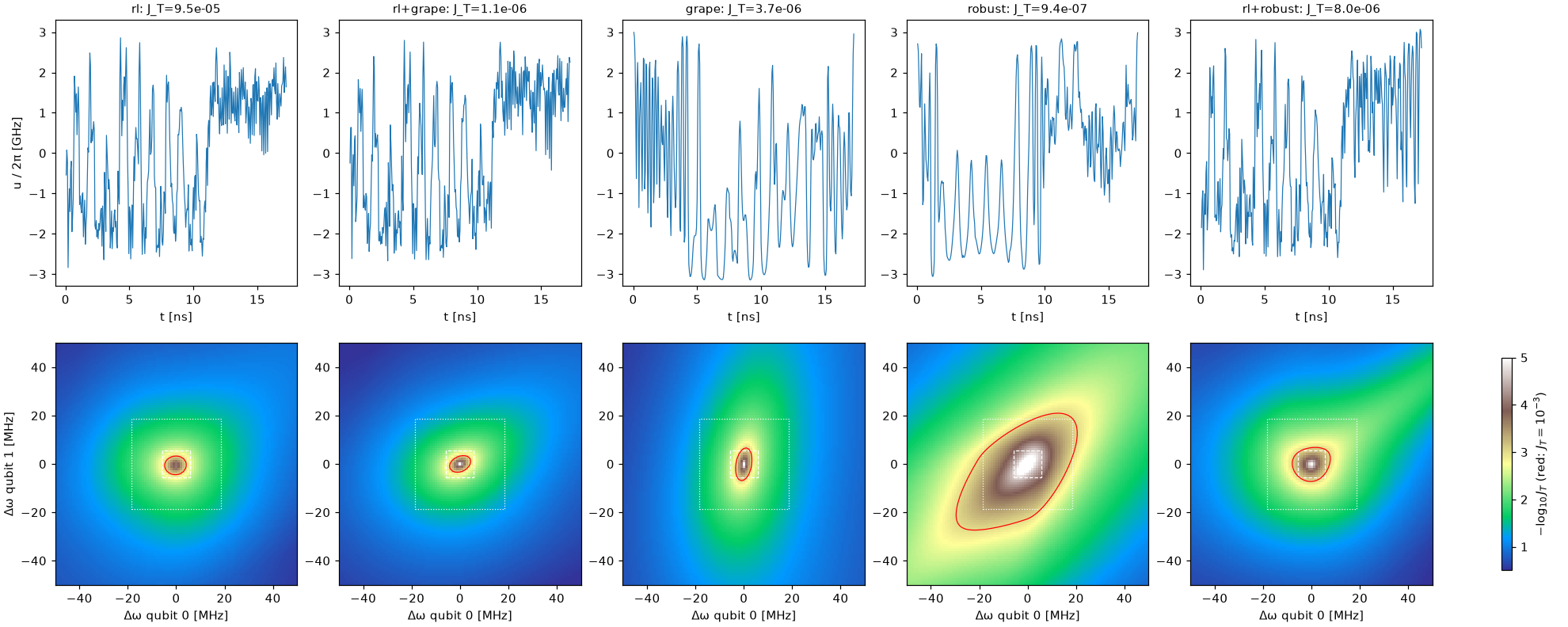
Top: pulses. Bottom: \(-\log_{10} J_T\) on the paper's ±50 MHz map; red contour at \(J_T = 10^{-3}\); white boxes: recool (dashed) and fabrication (dotted) ranges.

What the table says:

1. In-cooldown drift does not matter. Every pulse keeps its nominal J_T to within a factor of ~4 over ±0.1 MHz.
2. Recool drift is where pulses break. A single recool degrades the RL and GRAPE pulses from 1e-4-1e-6 to ~2e-3 on average.
3. RL's robustness is not special. RL, RL → GRAPE and plain GRAPE have the same recool mean, ~1.5-1.9e-3. The paper's comparison with Krotov was at a different gate time (50 ns) and bound (1.5 GHz).
4. Robust GRAPE wins on robustness, and it also has the best nominal J_T. Its mean over the fabrication range, which it never trained on, is 8.6e-4.
5. Starting robust GRAPE from the RL pulse is worse than from random guesses: the RL solution sits in a narrow basin.

GRAPE losses

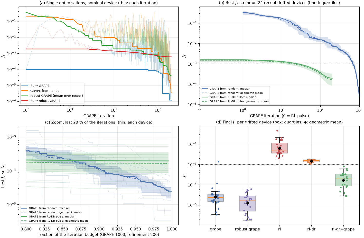
(a) The single optimisations of the table above: J_T at each iteration (thin) and best so far (thick); for robust GRAPE, the mean over the 25 systems. RL → GRAPE touches 1e-6. (b) Across the 24 drifted devices of the next section: median (solid), geometric mean (dashed) and quartile band of the best J_T so far. (c) Zoom on the last 20 % of the iterations, each device thin. (d) Final J_T on every drifted device for every method.

Refinement needs small steps

Started from the RL pulse with Adam at step 0.01 (as in the table), GRAPE first jumps out of the RL pulse's basin (J_T up to 5e-2) and only improves once the step has decayed, after ~600 iterations. With a step of 3e-4 it reaches J_T = 5e-7 in 50 iterations and 7e-9 in 200 from the paper's RL pulse. The per-device comparison below uses 3e-4.

RL vs GRAPE: cost per device

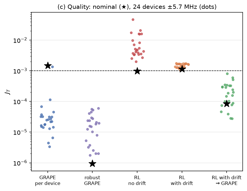
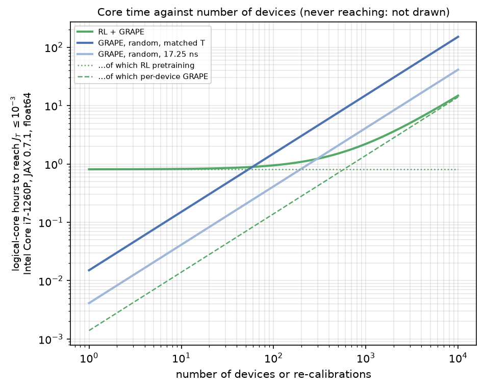
The question where RL can win: a device that is re-calibrated after every cooldown, or a fleet of devices, each with its own frequencies from the recool range. GRAPE pays its full cost for every device; a policy trained with domain randomisation pays once, then produces each device's pulse in a single rollout, and that pulse can seed a short GRAPE run.

Test set: the nominal device plus 24 devices with qubit frequencies drawn uniformly from the recool range (±5.7 MHz on each qubit), none of them seen in training. Target: J_T ≤ 1e-3. Both RL agents are PPO, seed 123, 20M steps; the drift-trained one redraws the qubit frequencies from the recool range every episode.

How compute is counted

Every cost on this page is logical-core time: the CPU time the computation takes on one logical core of the laptop's Intel i7-1260P, with JAX in float64. A job that keeps 16 logical cores busy for an hour counts as 16 core-hours. The costs are built from the steps each method actually took and the measured price of each step (scripts/bench_costs.py, one pinned logical core, single-threaded XLA):

Step	Core time at 2.1 GHz
One PPO environment step, including its share of the policy and value updates	145 µs (0.81 core-hours for 20M steps)
One GRAPE iteration, 17.25 ns pulse (345 samples), forward and backward	21 ms
Same, 35 ns / 50 ns pulse (700 / 1000 samples)	50 ms / 81 ms
One robust-GRAPE iteration, per ensemble member (345 samples)	10.4 ms
One policy rollout (333 steps)	25 ms

A laptop's clock swings tenfold with load and temperature (400 MHz to 4.7 GHz on this one; the benchmark ran at about 0.5 GHz while other training jobs throttled the chip). The benchmark therefore samples the core's clock during every measurement and quotes cycles as time at the 2.1 GHz base clock, so the numbers do not depend on how busy the machine was. At full turbo everything runs about twice as fast. Wall-clock times from the runs themselves are not used: they were measured on a shared, throttling machine with varying thread counts.

Click any figure to enlarge it; scroll or pinch to zoom.

Method	J_T nominal	J_T on drifted devices: median [quartiles]	Reaches 1e-3	One-off, core-hours	Per device, core-seconds
GRAPE per device (1000 iterations, random start)	1.5e-3*	2.4e-5 [1.5e-5, 3.2e-5]	96 %	0	14
Robust GRAPE (one pulse for all)	9.4e-7	1.7e-5 [4.9e-6, 2.8e-5]	100 %	0.58	0
RL trained without drift	9.8e-4	4.7e-3 [3.5e-3, 1.1e-2]	0 %	0.81	0.03 (one rollout)
RL trained with drift	1.2e-3	1.6e-3 [1.3e-3, 1.7e-3]	0 %	0.81	0.03 (one rollout)
RL with drift → 200 GRAPE steps	8.5e-5	2.0e-4 [8.6e-5, 3.3e-4]	100 %	0.81	0.94

* A single random restart on the nominal device happened to stall; the drifted devices show the typical GRAPE result.

Gate times differ in this comparison

The RL pulses here are cut at their best step, 38 ns in the median, while GRAPE from scratch runs at 17.25 ns, so the quality columns do not compare equal gate times. The fabrication-range control repeats GRAPE at matched gate times and finds the RL warm start still far better at equal budget.

What it shows:

1. Training with drift works as intended. The drift-trained agent's gates hardly change across devices (quartiles 1.3-1.7e-3), whereas the agent trained on one device degrades by 5× and scatters over a decade. The policy adapts; it just does not reach 1e-3 on its own.
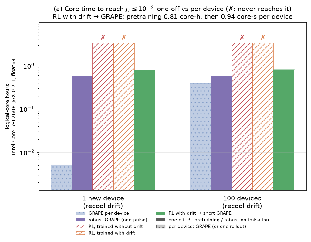
2. An RL pulse is a warm start that cuts GRAPE's compute per device 15×. From the drift-trained agent's pulse, about 16 small GRAPE steps (median) reach 1e-3 on every device: 0.94 core-seconds against 14 for GRAPE from a random guess. Each step is dearer (the RL pulse is 38 ns, 2.4× the samples of GRAPE's 17.25 ns), but far fewer are needed.
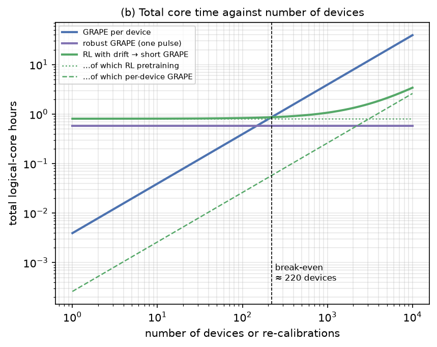
3. Amortisation pays off after ~220 devices. Training costs 0.81 core-hours once. Against GRAPE from scratch, RL + short GRAPE is cheaper after 0.81 h / (14 s − 0.94 s) ≈ 220 devices or recalibrations.
4. Within the recool range, one robust pulse is enough. Robust GRAPE's single pulse beats every per-device method on quality (median 1.7e-5) and needs nothing per device. Adaptation only matters when the drift is larger than what one pulse can cover.

Where RL should win, and the next experiment. Over the fabrication-targeting range (±18.5 MHz), robust GRAPE's worst case already degrades to 6.5e-3 (table above). That is where a policy that adapts per device, plus a short refinement, should beat both a single robust pulse and per-device GRAPE.

Fabrication-range experiment

The same comparison over the fabrication-targeting range (±18.5 MHz on each qubit): a PPO agent trained with drift redrawn every episode over ±0.35 % (±17.6 MHz and ±20.6 MHz on the two qubits), robust GRAPE on a 5 × 5 ensemble spanning ±18.5 MHz, and 24 held-out devices drawn from the range.

A single robust pulse still covers the whole range. Robust GRAPE trained over ±18.5 MHz:

Pulse	Nominal J_T	Recool: mean / worst	Fabrication: mean / worst	Optimisation, core-minutes
Robust GRAPE, recool ensemble (above)	9.4e-7	3.1e-5 / 1.4e-4	8.6e-4 / 6.5e-3	35
Robust GRAPE, fabrication ensemble	3.5e-5	3.7e-5 / 6.4e-5	1.0e-4 / 7.6e-4	35
RL → robust GRAPE, fabrication ensemble	1.9e-4	2.3e-4 / 4.2e-4	7.9e-4 / 4.1e-3	8.6

Trading a little nominal quality buys a pulse with J_T ≤ 7.6e-4 everywhere in the fabrication range. With two drifting frequencies, even ±18.5 MHz is not wide enough to need per-device adaptation in this model.

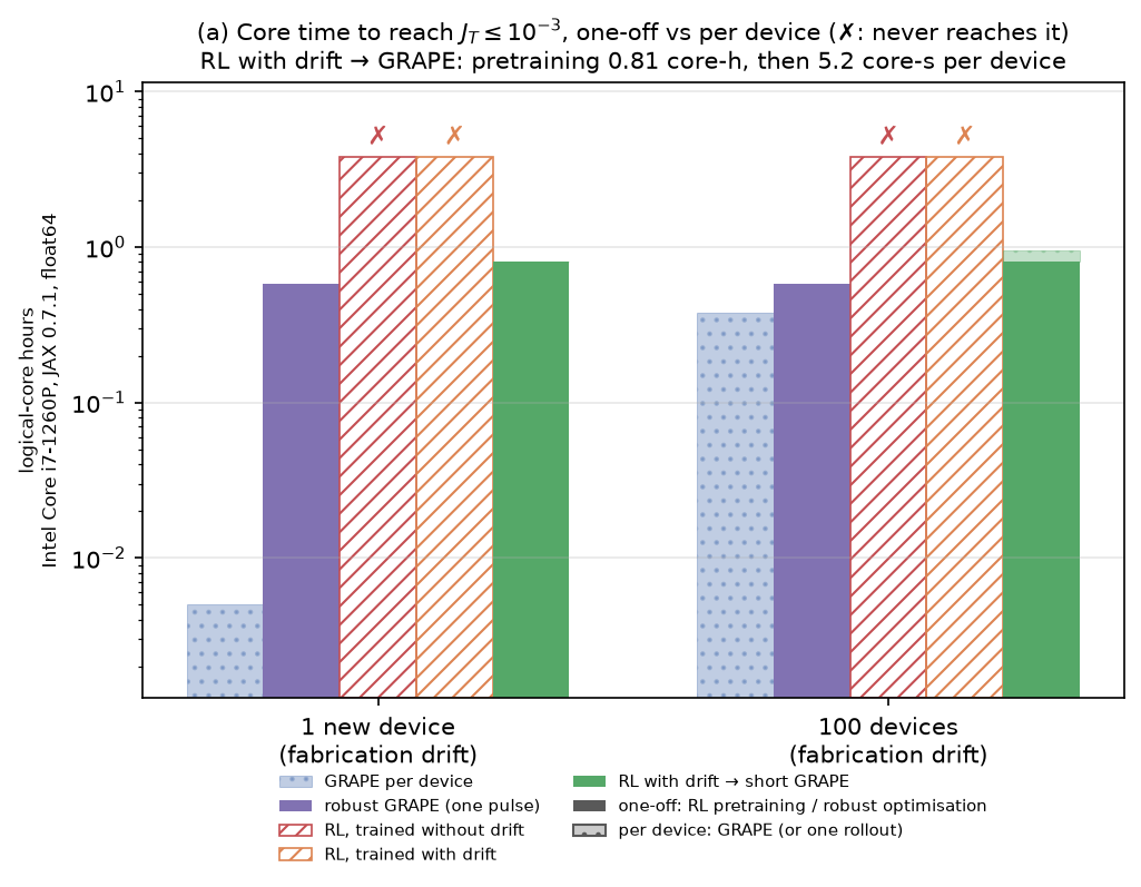
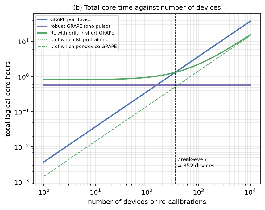
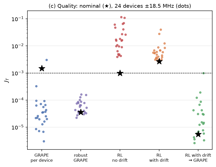
Click any figure to enlarge it; scroll or pinch to zoom.

Method	J_T on devices: median [quartiles]	Reaches 1e-3	One-off, core-hours	Per device, core-seconds
GRAPE per device (17.25 ns, random start)	3.1e-5 [1.9e-5, 6.5e-5]	96 %	0	13.5
Robust GRAPE, fabrication ensemble	5.5e-5 [3.4e-5, 8.1e-5]	100 %	0.58	0
RL trained without drift	1.6e-2 [8.4e-3, 4.3e-2]	0 %	0.81	0.03 (one rollout)
RL trained over the fabrication range	5.5e-3 [3.7e-3, 6.8e-3]	0 %	0.81	0.03 (one rollout)
RL (fabrication range) → 200 GRAPE steps	1.4e-5 [5.8e-6, 4.2e-5]	100 %	0.81	5.2 (until 1e-3)

The gate-time confound, and its control

The policy's pulse is cut at its best step, which here falls at 45 ns (median; quartiles 41-48 ns, docs/figures/gate_times.json), while GRAPE from scratch runs at 17.25 ns. A longer pulse gives GRAPE more freedom, so "RL → GRAPE beats GRAPE" could simply mean "a 45 ns pulse beats a 17 ns pulse". The control is GRAPE from a random guess at each device's own RL gate time (scripts/matched_gate_time.py):

GRAPE steps	Core-seconds per device (45 ns pulse)	From a random guess, matched gate time: median J_T (reach 1e-3)	From the RL pulse: median J_T (reach 1e-3)
50	3.6	4.9e-2 (0 %)	1.9e-3 (17 %)
100	7.1	3.0e-2 (0 %)	4.1e-4 (67 %)
200	14	1.3e-2 (0 %)	1.4e-5 (100 %)
500	36	6.6e-5 (96 %)	3.8e-8 (100 %)

At equal gate time and equal GRAPE budget the RL warm start is 1-3 orders of magnitude better, and it reaches the target in 200 steps where a random start needs close to 500. The warm start is genuinely informative, not an artefact of pulse length. A longer gate is itself a cost on hardware (more decoherence), which these closed-system numbers do not include.

Training and refinement budgets

J_T of the RL (fabrication range) policy at earlier checkpoints, alone and after 200 GRAPE steps:

Training	Core-minutes	Policy alone: median J_T	+ 200 GRAPE steps: median J_T	Reach 1e-3
2M steps	4.9	1.2e-2	7.3e-8	88 %
5M	12	8.4e-3	2.8e-4	79 %
10M	24	4.7e-3	1.8e-4	92 %
20M (final policy)	48	8.1e-3	1.2e-3	38 %

The policy's own quality improves up to 10M steps; the final policy had degraded (the late PPO instability seen in Training), so the best checkpoint should be used, as in the main table. The refined quality does not follow training monotonically: it depends on where each checkpoint's pulses end, i.e. on gate time. A policy trained for 2M steps (4.9 core-minutes, a tenth of the budget) is already a good warm start, which moves the break-even against per-device GRAPE from ~350 devices (full training) to about 36.

Where the per-device saving is smaller. On this range the warm start saves 2.6× per device (5.2 against 13.5 core-seconds), less than the 15× of the recool range. The policy's pulses are longer here (45 ns, 906 samples), and a GRAPE iteration on them costs 3.4× one on GRAPE's 17.25 ns pulse. The number of iterations falls ninefold (median 646 → 73); the price of each rises 3.4×. A policy trained with a gate-time penalty would recover much of the difference.

What the fabrication range shows

1. One robust pulse still suffices for two drifting frequencies, even over ±18.5 MHz.
2. The RL policy alone does not reach 1e-3 at this range, but it is a strong warm start: at equal gate time and GRAPE budget it beats a random start by 1-3 orders of magnitude.
3. Where RL can win is therefore not "one pulse per range" but "fast per-device refinement", and that advantage matters only when no single robust pulse covers the range, i.e. with more sensitive drifting parameters; see test T1.

Large coupler drift

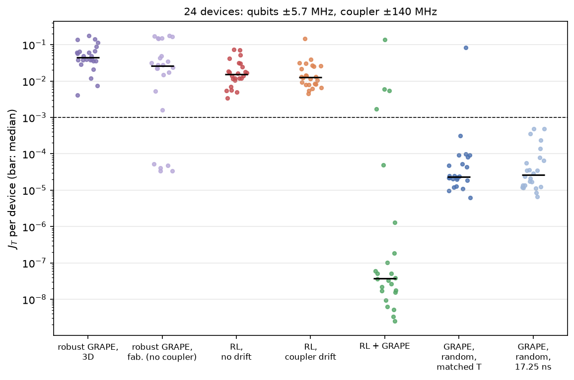
Qubits drifting over the recool range (±5.7 MHz each) and the coupler over ±140 MHz, the worst-loop flux drift after 17 days (Hardware drift ranges). Three drifting parameters, one of them very wide. Script: scripts/coupler_drift_experiment.py.

• Robust GRAPE, 3D: one 17.25 ns pulse optimised over 35 members (7 coupler offsets from −140 to +140 MHz × the centre and 4 corners of the qubit box), 2 restarts × 2000 iterations.
• PPO trained over the same drift (seed 123, 20M steps, drift redrawn every episode; best checkpoint at 7.8M steps), alone and as a warm start for 200 GRAPE steps.
• Controls: GRAPE from a random guess at each device's own RL gate time (matched) and at 17.25 ns, 1000 iterations each; the fabrication-range robust pulse, which never saw coupler drift.
• 24 held-out devices drawn uniformly from the 3D box. Target J_T ≤ 1e-3.

Method	J_T on devices: median [quartiles]	Reaches 1e-3	One-off, core-hours	Per device, core-seconds
Robust GRAPE, 3D ensemble	4.4e-2 [3.6e-2, 6.5e-2]	0 %	0.40	never reaches
Robust GRAPE, fabrication range (no coupler drift)	2.6e-2 [4.4e-3, 7.3e-2]	21 %	0.58	never reaches
RL trained without drift	1.5e-2 [1.1e-2, 2.6e-2]	0 %	0.81	never reaches
RL trained over the coupler drift	1.3e-2 [8.1e-3, 2.6e-2]	0 %	0.81	never reaches
RL (coupler drift) → 200 GRAPE steps	3.7e-8 [1.7e-8, 4.6e-7]	83 %	0.81	5.0
GRAPE, random start, matched gate time (46 ns), 1000 steps	2.3e-5 [1.9e-5, 6.0e-5]	96 %	0	54
GRAPE, random start, 17.25 ns, 1000 steps	2.7e-5 [1.3e-5, 6.9e-5]	100 %	0	15

Per-device core time is to the first iteration below 1e-3 (median over devices). The policy's gates last 46 ns in the median (quartiles 37-49 ns).

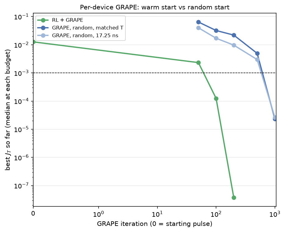
GRAPE steps	RL warm start: median J_T (reach 1e-3)	Random, matched gate time	Random, 17.25 ns
0	1.3e-2 (0 %)
50	2.3e-3 (29 %)	6.4e-2 (0 %)	4.0e-2 (0 %)
100	1.3e-4 (83 %)	3.2e-2 (0 %)	1.7e-2 (0 %)
200	3.7e-8 (83 %)	2.2e-2 (0 %)	9.7e-3 (0 %)
500		4.9e-3 (4 %)	3.0e-3 (13 %)
1000		2.3e-5 (96 %)	2.7e-5 (100 %)

What large coupler drift shows

1. For the first time, one pulse does not cover the range. Robust GRAPE cannot even fit its own 35 members (mean J_T 2.7e-2 over the ensemble) and reaches 1e-3 on none of the held-out devices. The fabrication-range robust pulse reaches it only on the 5 devices whose coupler sits within 11 MHz of nominal, consistent with its 64 MHz-wide coupler window in the coupler scan (narrower here, where the qubits drift too). This is the regime the hypothesis is about.
2. The policy alone is not enough either. Trained over the drift or not, it gives J_T ≈ 1e-2: the drift-trained policy is barely better, so at this width the policy has not learned to compensate the coupler by itself.
3. But its pulse is a very strong warm start. 100 GRAPE steps from it reach 1e-3 on 83 % of the devices; from a random start at the same gate time, 100 steps reach none, and 1000 are needed. Where it converges, the refined gate is three orders of magnitude better than GRAPE from scratch (median 3.7e-8 vs 2.3e-5). On 4 of 24 devices the warm start stalls above 1e-3 within 200 steps, with no pattern in their coupler offsets (+120, −99, −87 and −9 MHz).
4. Compute. Per device, RL + GRAPE takes 5.0 core-seconds against 54 for GRAPE at matched gate time and 15 for GRAPE at 17.25 ns. The 0.81 core-hours of training pay back after ≈ 60 devices against the matched control and ≈ 300 against 17.25 ns GRAPE.

What this does not show yet

The robust pulse was optimised at 17.25 ns, while the policy's pulses run 46 ns. A longer robust pulse has more freedom and might cover the range; until that is tested, "no single pulse suffices" holds at 17.25 ns only. Robust GRAPE was also given only 35 members and 2 restarts. The next runs: robust GRAPE at 46 ns with more members, and more restarts for the 4 devices where refinement stalls.

The same experiment with a √iSWAP gate-fidelity target and measurable observations is on Measurable observations and gate fidelity: the conclusions hold, and the policy on its own adapts better.

The robust optimisation took about 66 minutes of wall time on the shared machine (from file timestamps; the script did not wait for the asynchronous JAX result, since fixed); the core-hours above come from its iteration count.