The calibration policy: a new MDP

The paper's agent builds a pulse sample by sample and watches the quantum state while it does. That works in simulation, but on hardware the state is not observable, a gate must survive drift, and every observation costs shots. Ideas gecko, ibis and jackal change the decision problem step by step. This page describes where it has arrived, the carrier calibration MDP, and why each change was made.

What changed, in one table

	Paper (v1)	Calibration policy (ibis, jackal)
What the agent observes	The quantum state: 12 complex amplitudes of the evolving computational states (not measurable)	A calibration of the device, measured once before the pulse: the offsets of both qubit frequencies and the coupler frequency from nominal, in MHz, as spectroscopy gives them (with measurement error). Plus its own knobs and the time
Observation size	28	8: 3 calibration numbers, 4 knob values (A, b, cos φ, sin φ), time
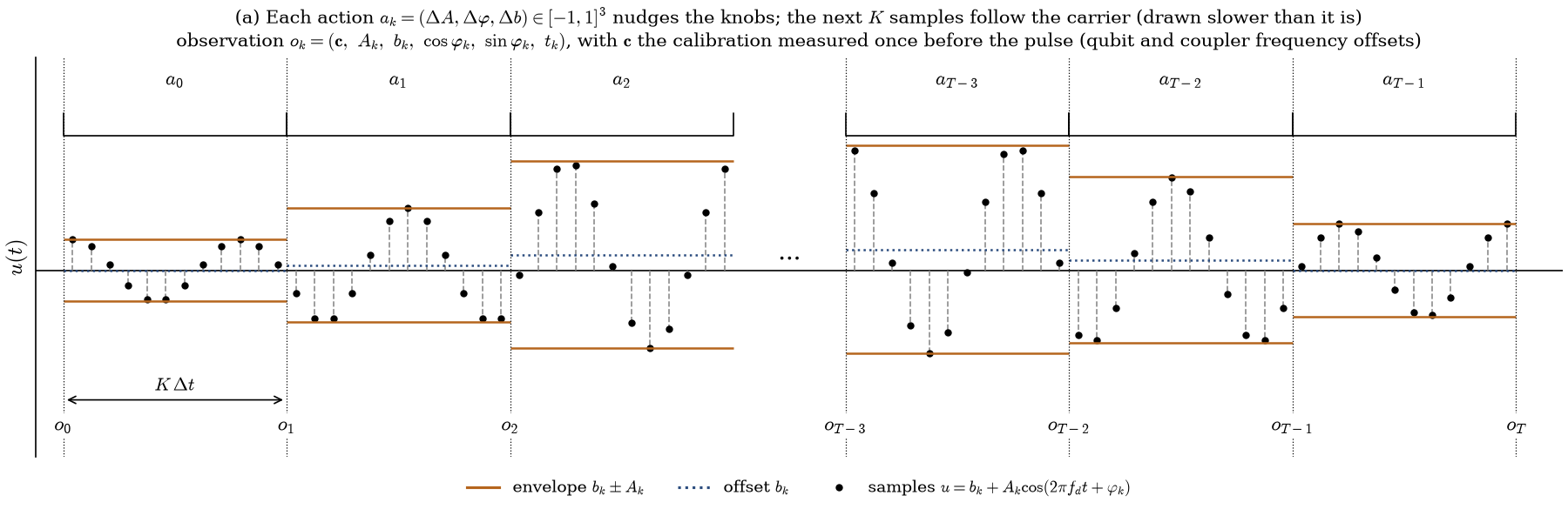
What an action is	3 per-sample amplitude changes Δu, summed into the pulse	3 knob changes (ΔA, Δφ, Δb) of a carrier u(t) = b + A cos(2π fd t + φ)
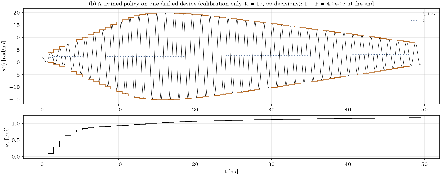
Pulse between decisions	Piecewise constant, 3 samples	The carrier with the current knobs, K samples (15 in the best ibis policy, 50 of 0.1 ns on the device)
Carrier frequency fd	none	The qubit-qubit detuning as measured by the calibration (nominal + measured offsets)
Decisions per pulse	333	66 (ibis, K = 15); 20 (jackal, 100 ns)
Amplitude bound	Leaving it ends the episode	Clipped, with a penalty on the excess
Reward	−log10 JT (perfect entangler) per step	−log10(1 − F) per step, F the average gate fidelity to √iSWAP after free virtual-Z corrections, leakage included
Loop at deployment	Closed loop on the state	Open loop: calibrate, roll the policy out, play the pulse
Data per pulse on hardware	Not possible (the state is not observable)	One calibration, about 1e4 shots

How a pulse is built

At each decision point o_k the policy sees the calibration, its current knobs and the time, and outputs a_k = (ΔA, Δφ, Δb) ∈ [−1, 1]³, scaled to at most (1 rad/ns, 0.2 rad, 1 rad/ns) in ibis. The next K samples follow the carrier with the updated knobs. The carrier runs in absolute time, so it stays continuous across decisions; only a change of phase or amplitude makes a small step at the boundary. Compare the paper's per-sample actions (home page).

What a trained ibis policy (calibration only, K = 15) plays on one of the held-out drifted devices: the envelope b ± A (orange), the offset b (blue, dotted), the pulse (black) and the phase φ. It ramps the amplitude up to the bound within about 15 ns, holds it, and ramps it down; it moves the phase by about 1 rad in the first 5 ns (a small shift of the effective frequency) and keeps a small offset of 2-3 rad/ns. The final gate on this device: 1 − F = 4.0e-3.

Training and deployment

flowchart LR
    subgraph T[Training, in simulation]
        direction TB
        S1[Draw a device:<br/>qubit, coupler drift] --> S2[Calibration:<br/>true offsets + measurement error]
        S2 --> S3[Policy: o_k = calibration, knobs, t<br/>a_k = knob changes]
        S3 --> S4[Simulator plays the<br/>next K samples]
        S4 -->|reward: -log10 1-F| S5[PPO update]
        S4 -->|next decision| S3
    end
    subgraph D[Deployment, on a device]
        direction TB
        D1[Spectroscopy:<br/>qubit and coupler frequencies] --> D2[Policy rolled out<br/>deterministically, offline]
        D2 --> D3[Waveform:<br/>carrier with the knob sequence]
        D3 --> D4[AWG plays the pulse:<br/>the gate]
    end
    T -. trained weights .-> D

The simulator is only used in training: it supplies the reward and plays the pulse. At deployment nothing is measured during the pulse. The policy never sees the Hamiltonian, the fidelity or the state, only the calibration, so the same weights work on any device whose calibration it can read. What it can not see (drift of the couplings or anharmonicities, a stale calibration) is tested separately on the ibis page.

Why these changes

1. Observe the device, not the state. The right pulse depends only on the device, which does not change during the pulse. Observing the evolving state (the paper's choice) makes the policy a feedback controller that needs a measurement at every step: 1e7 shots per pulse, and with finite shots it falls apart (30× worse at 1e6 shots). A calibration is measured anyway, once, and is enough.
2. Steer slow knobs, not samples. A good pulse rides on a carrier near the qubit detuning (0.86 GHz in the paper's model, 43 periods in 50 ns). A policy that only sees a clock cannot synthesise that carrier sample by sample: with per-sample actions and calibration-only observations it stayed at the identity gate for 20M steps. With the carrier given, it reached 1e-2 in 0.72M steps. It is also how gates are driven in a lab: a calibrated carrier with shaped envelope and phase.
3. Few, long steps. 66 decisions learn well; 333 small knob decisions learn badly or not at all.
4. Keep the pulse. Clipping with a penalty replaces ending the episode at the amplitude bound, so a single overshoot no longer destroys a device's gate.
5. A fidelity a lab reports. The average gate fidelity to √iSWAP with free Z (virtual Z gates cost nothing on hardware), instead of "any perfect entangler".

In the code

cfg = EnvConfig(objective="sqrt_iswap", obs_mode="context", action_mode="carrier",
                oob_mode="clip", n_time_steps=15)                       # ibis
cfg = EnvConfig(physics_model="device", obs_mode="context", action_mode="carrier", ...)   # jackal

CLI: --objective sqrt_iswap --obs-mode context --action-mode carrier --oob-mode clip --n-time-steps 15, or --physics device for the realistic model. The step with the carrier is in env.py (step, action_mode == "carrier") and env_device.py; the calibration is built in reset_params.