🦄 i08 hippogriff: know the device first, then act
🟢 active toy stage concluded in v2.18.1 · next: the gate step on jackal's realistic device model
Question. Merge dragonfly's structure (a latent, caution, directed exploration) with fox's empiricism. On a new device, can an agent first identify the drift, with an uncertainty that is largest at the first action and shrinks with every interaction, and then act on what it has learned, instead of re-training? (A hippogriff is the offspring of a griffin and a horse: a hybrid of a hybrid.)
Answer so far. Yes, on the toy devices. Identifying the drift lifts the first-episode return from 327 (a robust policy) to 614-627 of the oracle's 655, where black-box fine-tuning (fox) barely recovered after 60 updates. The first belief, a linearised Kalman filter, became badly overconfident (its uncertainty shrank around a wrong value); an exact grid belief fixes that and is robust to noise and to a learned measurement model, and a consistency check lets the Kalman belief recover to the oracle with the exact model. Probing for information pays where the belief is weak.
The key idea: a belief that can only sharpen
A model that imagines a rollout (chameleon, dragonfly) accumulates error with every imagined step. Deployment is different: every real interaction adds information. With a Gaussian belief \(\mathcal N(m, P)\) over the drift z and each interaction treated as a (linearised) measurement \(y = h(s, a, z) + \text{noise}\), the Kalman update
can only shrink the uncertainty. Autoregression here is over interactions (the belief is recursive), not over action dimensions (axolotl's mistake), and the only structure the policy and the model share is the drift latent z.
Design (hippogriff.py, toy_envs.DriftTracker)
Stage 1, simulation.
- PPO with domain randomisation over the drift range, the policy conditioned on the drift: \(\pi(a \mid s, z)\), z the device's normalised (gain, offset) in \([-1, 1]^2\).
- A blind control that never sees z: the classic robust policy.
- Fox's improvement model rides along during PPO (no exploitation), and its calibration is logged.
Stage 2, deployment, the drift unknown:
- The belief starts at the prior (the whole range: mean 0, variance 1/3 per dimension) and is updated after every step by an extended Kalman filter (Joseph form), with the measured change of the commanded amplitude and the tracking score as y.
- The measurement model is either the environment's own differentiable
measure(A, grey box: the physics is known, only its parameters drift, and J comes from autodiff through the simulator), or a network trained on simulated transitions (B, black box; its R from held-out residuals). - Trust region: actions are clipped to \(c = c_\min + (1 - c_\min)(1 - \rho)\), with \(\rho = (\det P / \det P_0)^{1/2d}\): small first actions, widening as the uncertainty shrinks.
- Safety: a candidate action is vetoed if the model predicts an overshoot at any sigma point of the belief.
- Probing: while \(\rho > 0.1\), the candidate with the largest expected information gain, \(\tfrac12 \log\det(I + R^{-1} J P J^\top)\), is chosen. Afterwards, \(\pi(a \mid s, m)\).
Modes compared on the same held-out devices as fox: blind, robust (z fixed at the prior mean), oracle (true z), filter (the belief updates z, actions from π: passive identification) and hippogriff (filter + trust region + safety + probing), each filter with model A and B.
Smoke test (1 seed, 4 devices, 300k pretraining steps, 3 episodes per device)
| Mode | Episode 1 | Episodes 2-3 | Drift error after episode 1 |
|---|---|---|---|
| blind | 314 | 312-314 | – |
| robust | 305 | 303-306 | 0.85 |
| filter A | 463 | 461-465 | 0.000 |
| hippogriff A | 461 | 461-465 | 0.000 |
| filter B | 461 | 462-465 | 0.084 |
| hippogriff B | 456 | 462-465 | 0.085 |
| oracle | 464 | 461-465 | – |
The learned measurement model (B) explains 97-99.9 % of the variance of its outputs on held-out transitions. Fox's model, monitoring pretraining, predicted return changes early in training (correlation 0.30-0.36 with the realised change) but not near convergence (−0.08 to −0.30 in the second half).
Full results (3 seeds × 12 devices × 5 episodes, 2M pretraining steps)
Noise-free measurements, and noisy ones (amplitude change ± 0.02, tracking score ± 0.5, like finite shots on hardware; the filter knows the noise level). Return per episode is the mean over the 12 devices.
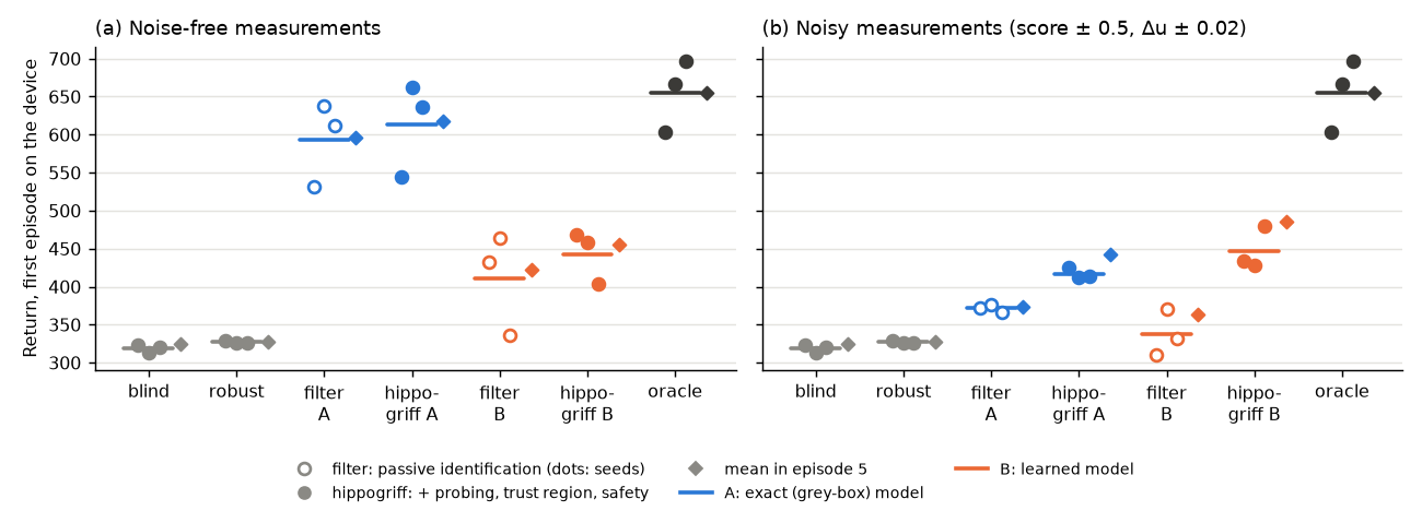
| Mode | Noise-free: episode 1 (seeds) | episode 5 | Noisy: episode 1 (seeds) | episode 5 |
|---|---|---|---|---|
| blind | 319 (324, 314, 321) | 324 | same as noise-free | |
| robust | 327 (329, 326, 326) | 327 | same | |
| filter A | 593 (531, 638, 611) | 596 | 372 (373, 376, 367) | 373 |
| hippogriff A | 614 (544, 662, 636) | 617 | 417 (425, 413, 414) | 442 |
| filter B | 411 (432, 464, 336) | 423 | 337 (310, 371, 331) | 364 |
| hippogriff B | 443 (468, 458, 403) | 455 | 447 (434, 429, 480) | 486 |
| oracle | 655 (603, 666, 696) | 655 | same |
(The blind, robust and oracle modes do not measure anything, so noise does not affect them.)
- Knowing the device is worth almost everything. With the exact model (A) and clean measurements, identification recovers 614 of the oracle's 655, against 327 for the robust policy.
- Probing earns its keep, the more so the harder identification is: +21 (A) and +32 (B) without noise; +45 (A) and +110 (B) with noise, where passive operation reveals the drift only slowly. With noise the full method probes for 7-8 steps (A) or 21-23 steps (B) of the first episode, against about 2 without.
- The learned model (B) wins under noise (447 vs 417). Its R includes its own fitting error, so it trusts each measurement less, which turns out to be the right thing to do (next section).
The flaw: a belief that shrinks around the wrong value
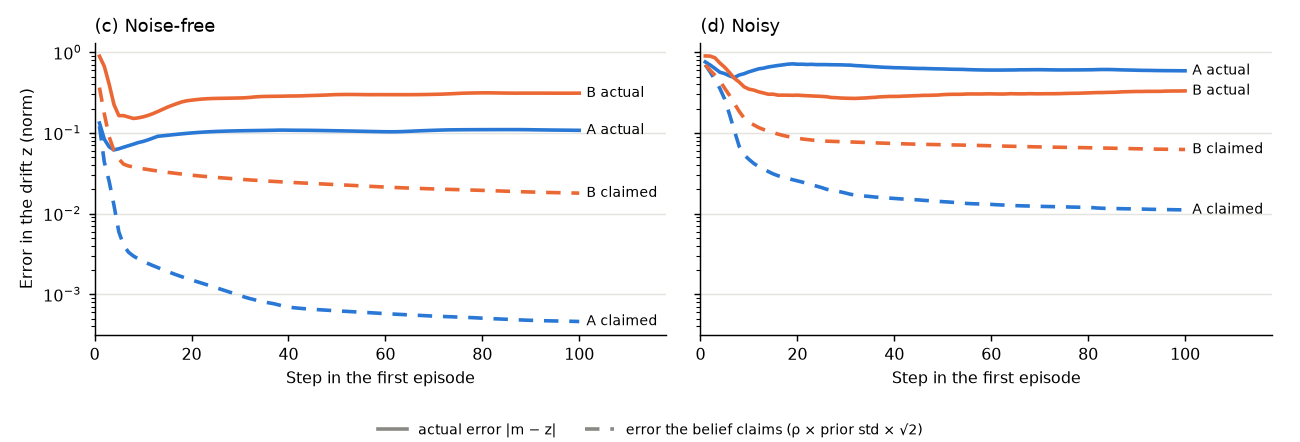
| After 5 episodes | Actual error in z | Error the belief claims | Overconfident by |
|---|---|---|---|
| hippogriff A, noise-free | 0.12 | 0.0002 | ×680 |
| hippogriff B, noise-free | 0.36 | 0.008 | ×43 |
| hippogriff A, noisy | 0.54 | 0.003 | ×170 |
| hippogriff B, noisy | 0.34 | 0.036 | ×9 |
The Kalman update guarantees that the reported uncertainty shrinks. It does not guarantee that the estimate is right. In the noise-free case the actual error drops to about 0.06 within three steps and then rises again while the claimed error keeps falling: the filter talks itself into a wrong answer and, with its uncertainty already tiny, no later measurement can move it. The cause is the linearisation: the tracking score, \(-\log_{10}( ext{error})\), is far from linear in the drift, so a first-order update is confidently wrong. That is why the learned model, with its larger R, does better under noise.
Fixing the belief: three filters on the same policies
Same pretrained policies and devices, three beliefs (--set filter=...):
ekf: the linearised Kalman filter above.ekf_nis: the same, with a consistency check. When a measurement is more surprising than the belief allows (normalised innovation squared above the 99 % χ² bound), the uncertainty is scaled up before the update (at most back to the prior). This is the "artificial confidence bound" used as a floor.grid: exact Bayes on a 41 × 41 grid over the drift; no linearisation. Probing uses the spread of the model's predictions over the whole belief, which reduces to the Jacobian formula for a linear model.
Return per episode (mean over 12 devices and 3 seeds; oracle 655, robust 327, blind 319), and the error in the drift after 5 episodes:
| Belief | Model | Noise-free: filter / hippogriff, episode 1 → 5 | error | Noisy: filter / hippogriff, episode 1 → 5 | error |
|---|---|---|---|---|---|
ekf |
A (exact) | 593 → 596 / 614 → 617 | 0.17 / 0.12 | 372 → 373 / 417 → 442 | 0.70 / 0.54 |
ekf_nis |
A | 600 → 655 / 610 → 655 | 0.00 / 0.00 | 400 → 634 / 395 → 570 | 0.05 / 0.19 |
grid |
A | 627 → 627 / 622 → 626 | 0.05 / 0.06 | 575 → 629 / 591 → 622 | 0.06 / 0.06 |
ekf |
B (learned) | 411 → 423 / 443 → 455 | 0.49 / 0.36 | 337 → 364 / 447 → 486 | 0.62 / 0.34 |
ekf_nis |
B | 214 → 228 / 271 → 320 | 1.46 / 0.75 | 270 → 272 / 398 → 453 | 1.20 / 0.13 |
grid |
B | 541 → 540 / 549 → 548 | 0.27 / 0.29 | 530 → 539 / 511 → 546 | 0.23 / 0.21 |
- The exact grid belief is the robust choice: best or close to best in the first episode in every setting, and noise barely hurts it (575-591 against 622-627 noise-free). With the learned model it lifts the first episode from 337-486 (EKF) to 511-549.
- The consistency check lets a belief recover from a wrong early commitment: with the exact model the
ekf_nisbelief reaches the true drift and the oracle's 655 by episode 5, which the plain EKF never does. But it is slow in the first episode, and it breaks with the learned model: the model's own errors look like surprises, the belief keeps inflating and ends further from the truth than the prior (error 1.2-1.5 against 0.85). - Probing matters where the belief is weak. It added +21 to +110 for the EKF; with the grid belief, ordinary operation is already informative and probing changes the first episode by −19 to +16.
- What is left: the grid's resolution (spacing 0.05 in z, an error floor about 0.05) for model A, and the learned model's bias (error 0.2-0.3) for model B.
Which run is which
Everything is in runs/i08_hippogriff/ (gitignored); the summaries are in results/i08_hippogriff/.
| Directory | What it is |
|---|---|
pretrained/seed{0,1,2}_2000000.pkl |
the cached stage-1 artefacts per seed: z-conditioned and blind PPO policies, learned model B; every variant below deploys these |
seed{s}_20260925-2136xx_ekf / _ekf_noisy |
the linearised Kalman belief, noise-free / noisy (the "Full results" above) |
seed{s}_20260925-2136xx_nis / _nis_noisy |
the Kalman belief with the consistency check |
seed{s}_20260925-2136xx_grid / _grid_noisy |
the exact grid belief |
logs/ |
the console logs (full_*, noisy_*: the first runs; filters_*: the comparison) |
Each variant directory holds results.json with all 7 modes (blind, robust, oracle, filter A/B,
hippogriff A/B): returns per episode and device, and the belief's error and ρ at every step. The first
full runs (seed*_20260925-2030xx, …-2039xx_noisy) were exact duplicates of the ekf variants and are
archived in runs/_attic/.
Next
- The gate environment with a particle belief over the physical drift (qubit and coupler frequencies, couplings): each particle simulates its own device through the same actions, since the quantum state depends on the drift. Ibis has since found that a policy fed a routine frequency calibration plays a good pulse open loop; hippogriff's question there becomes whether identification during operation can replace, or refine, that calibration, and catch the drift the calibration does not see (couplings, anharmonicities), which jackal (i10, in progress) also tests.
- A finer or adaptive grid (or particles) to remove the resolution floor.
Fox's improvement model, riding along during the 2M-step pretraining, predicted each update's return change only weakly (correlation 0.07-0.15 with the realised change for the drift-conditioned policy, 0.03-0.09 for the blind one).
Records: results/i08_hippogriff/summary.json; figures from scripts/plot_hippogriff.py
(data in docs/figures/hippogriff.json).
Rerun: python -m rlquantopt.jx.hippogriff --seed 0 --devices 12 --episodes 5 [--set noise_du=0.02 noise_score=0.5 --tag noisy].